
“Development of a Python program for investigation of reaction-diffusion coupling in oscillating reactions”
Github
Introduction
The Brusselator is a model developed by I. Prigogine and R. Lefever at the Universite Libre de Bruxelles in Belgium. [16] developed for the description of nonlinear systems. The model includes some assumptions [12, 11], such as irreversible reactions ( for
for  and constant reactant and product species concentrations A, B, C and D. Realistically, this happens by constant addition of A and B and removal of C and D.
![\[\ce{A} \ce{->[k_1]} \ce{X}\]](https://lukaswittmann.com/wp-content/ql-cache/quicklatex.com-b51df4ea95870c437a6fb1ac003422fa_l3.png "Rendered by QuickLaTeX.com")
![\[\ce{B + X} \ce{->[k_2]} \ce{Y + D} \]](https://lukaswittmann.com/wp-content/ql-cache/quicklatex.com-ab979241364b59f3d95859fa313a9f27_l3.png "Rendered by QuickLaTeX.com")
![\[\ce{2 X + Y} \ce{->[k_3]} \ce{3 X} \]](https://lukaswittmann.com/wp-content/ql-cache/quicklatex.com-ebd20247b6cb850f71ed78d6f341fcee_l3.png "Rendered by QuickLaTeX.com")
![\[\ce{X} \ce{->[k_4]} \ce{E} \]](https://lukaswittmann.com/wp-content/ql-cache/quicklatex.com-3d6f0a7a358e71ec24f54f0b43634725_l3.png "Rendered by QuickLaTeX.com")
![\[\_\_\_\_\_\_\_\_\_\_\_\_\_\_\_\_\_\_\_\_\_\_\]](https://lukaswittmann.com/wp-content/ql-cache/quicklatex.com-a3d6399df47726a5138e62700feced9b_l3.png "Rendered by QuickLaTeX.com")
![\[\ce{A + B} \ce{->} \ce{D + E}\]](https://lukaswittmann.com/wp-content/ql-cache/quicklatex.com-840ed004d980274718aff14de96a1ab6_l3.png "Rendered by QuickLaTeX.com")
With the assumptions of chapter 2.1, the dierential kinetic time laws of the species X and Y can be derived. The concentration of a species is noted with square brackets. The concentration notation is assumed to be dimensionless in the following, since there is a mathematical consideration of the issue. With ![[D]=[E]=0](https://lukaswittmann.com/wp-content/ql-cache/quicklatex.com-190f663d83a348bdb24f4c4c2d3d1a6b_l3.png "Rendered by QuickLaTeX.com") and for
and for  the differential time laws follow.
![\[f\left([X],[Y]\right) \;\equiv\; \dfrac{\text{d} \left[X\right]}{\text{d} t} = k_1 \left[A\right] - k_2 \left[B\right] \left[X\right] + k_3 \left[X\right]^2 \left[Y\right] - k_4 \left[X\right] \label{eq_DGL_f}\]](https://lukaswittmann.com/wp-content/ql-cache/quicklatex.com-bcdd9dd9ef8f5f40461fc21644ca080d_l3.png "Rendered by QuickLaTeX.com")
![\[g\left([X],[Y]\right) \;\equiv\; \dfrac{\text{d} \left[Y\right] }{\text{d} t} = k_2 \left[B\right] \left[X\right] - k_3 \left[X\right]^2 \left[Y\right] \label{eq_DGL_g}\]](https://lukaswittmann.com/wp-content/ql-cache/quicklatex.com-6a8b07a3488a2be80a128220a6c3032b_l3.png "Rendered by QuickLaTeX.com")
Spatially Homogeneous Brusselator
Dynamic Analysis of the Spatially Homogeneous Brusselator
This part is rather long and thus shortened. The full version is shown in detail in my thesis. The fixpoint can be calculated. ![\[\left[X \right]^* = \dfrac{k_1 \left[A\right]}{k_4} \label{eq_fixpunkt_X}\]](https://lukaswittmann.com/wp-content/ql-cache/quicklatex.com-efae9047a7b95e8cf0c5ec198238e182_l3.png "Rendered by QuickLaTeX.com")
![\[\left[Y \right]^* = \dfrac{k_2 k_4 \left[B\right]}{k_3 k_1 \left[A\right]} \]](https://lukaswittmann.com/wp-content/ql-cache/quicklatex.com-bb16821bb391fba08c6d36eb24bafda6_l3.png "Rendered by QuickLaTeX.com")
![\[ F=\left(\dfrac{k_1 \left[A\right]}{k_4} ,\; \dfrac{k_2 k_4 \left[B\right]}{k_3 k_1 \left[A\right]}\right)\]](https://lukaswittmann.com/wp-content/ql-cache/quicklatex.com-2d8ba8e25b2c5076411d31d4aa8e20f7_l3.png "Rendered by QuickLaTeX.com")
![\[U = [X] - [X]^* \]](https://lukaswittmann.com/wp-content/ql-cache/quicklatex.com-541e32ebc9af7728ed8c831b1ec7402e_l3.png "Rendered by QuickLaTeX.com")
![\[V = [Y] - [Y]^* \]](https://lukaswittmann.com/wp-content/ql-cache/quicklatex.com-3ede706b40c7ec4f38945e634c06f282_l3.png "Rendered by QuickLaTeX.com")
![\[\dfrac{\text{d} U}{\text{d} t}= \dfrac{\text{d} [X]}{\text{d} t} \]](https://lukaswittmann.com/wp-content/ql-cache/quicklatex.com-4c08d4d5d3af9ff6fd1c0a5b71f05dab_l3.png "Rendered by QuickLaTeX.com")
![\[\dfrac{\text{d} V}{\text{d} t} = \dfrac{\text{d} [Y]}{\text{d} t} \]](https://lukaswittmann.com/wp-content/ql-cache/quicklatex.com-6ee37f2cbce012b305a027ad31b37380_l3.png "Rendered by QuickLaTeX.com")
![f\left([X],[Y]\right)](https://lukaswittmann.com/wp-content/ql-cache/quicklatex.com-375a88df55966aa61e5779c413bfac5b_l3.png "Rendered by QuickLaTeX.com") and
and ![g\left([X],[Y]\right)](https://lukaswittmann.com/wp-content/ql-cache/quicklatex.com-e05aae941fa2e582aecaca11da256701_l3.png "Rendered by QuickLaTeX.com") are substituted and a Taylor series approximation is used.
are substituted and a Taylor series approximation is used.
![\[\dfrac{\text{d} U}{\text{d} t} = f\left([X]^* + U, [Y]^* + V\right) = f([X]^*,[Y]^*) + U\dfrac{\delta f([X]^*,[Y]^*)}{\delta [X]}+ V\dfrac{\delta f([X]^*,[Y]^*)}{\delta [Y]} + h\left(U^2,V^2,UV\right)\]](https://lukaswittmann.com/wp-content/ql-cache/quicklatex.com-4b24925a83df79481fcaa60d29543748_l3.png "Rendered by QuickLaTeX.com")
 .
.
![\[\dfrac{\text{d} U}{\text{d} t} = U\dfrac{\delta f([X]^*,[Y]^*)}{\delta [X]}+ V\dfrac{\delta f([X]^*,[Y]^*)}{\delta [Y]} + h\left(U^2, V^2, UV\right) \]](https://lukaswittmann.com/wp-content/ql-cache/quicklatex.com-6ff6ba5e12da730e0e9b15ec0239d159_l3.png "Rendered by QuickLaTeX.com")
![\[\dfrac{\text{d} V}{\text{d} t} = U\dfrac{\delta g([X]^*,[Y]^*)}{\delta [X]}+ V\dfrac{\delta g([X]^*,[Y]^*)}{\delta [Y]} + h\left(U^2, V^2, UV\right)\]](https://lukaswittmann.com/wp-content/ql-cache/quicklatex.com-31b0e18110c695b2911369c42d2a71e9_l3.png "Rendered by QuickLaTeX.com")
 ) it is obvious, that the matrix of partial derivatives is the Jacobian. This is only possible as long as the position and type of the fixed point of the linearized system is also exactly the one of the non-linear system.
![\[\renewcommand{\arraystretch}{2} \begin{bmatrix} \dfrac{\text{d} U}{\text{d} t} \\ \dfrac{\text{d} V}{\text{d} t} \end{bmatrix} = \begin{bmatrix} \dfrac{\delta f}{\delta \left[X\right]} \dfrac{\delta f}{\delta \left[Y\right]} \\ \dfrac{\delta g}{\delta \left[X\right]} \dfrac{\delta g}{\delta \left[Y\right]} \end{bmatrix} \begin{bmatrix} U \\ V \end{bmatrix}= J_{g,f}\left(\left[X\right],\left[Y\right] \right) \begin{bmatrix} U \\ V \end{bmatrix} = \begin{bmatrix} - k_2 \left[B\right] + 2 k_3 \left[X\right]\left[Y\right] - k_4 & k_3 \left[X\right]^2 \\ k_2 \left[B\right] - 2 k_3 \left[X\right]\left[Y\right] & - k_3 \left[X\right]^2 \end{bmatrix}\begin{bmatrix} U \\ V \end{bmatrix}\]](https://lukaswittmann.com/wp-content/ql-cache/quicklatex.com-45a2216b13773039447b14bca6aed1c7_l3.png "Rendered by QuickLaTeX.com")
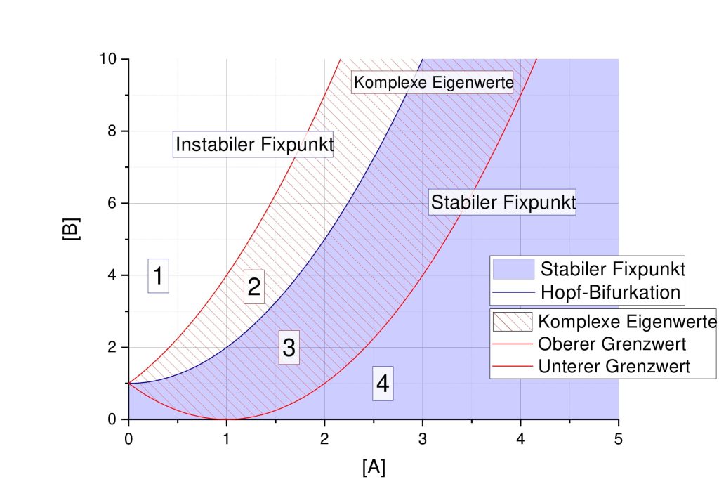
![\[\lambda_{1,2}=\left[ \begin {array}{c} {\dfrac {-{[A]}^{2}+[B]-1}{2}}+{\dfrac {1}{2}\sqrt {{[A]}^{4}-2\,{[A]}^{2}[B]-2\,{[A]}^{2}+{[B]}^{2}-2\,[B]+1}}\\ \dfrac {-{[A]}^{2}+[B]-1}{2}+{\dfrac {1}{2}\sqrt {{[A]}^{4}-2\,{[A]}^{2}[B]-2\,{[A]}^{2}+{[B]}^{2}-2\,[B]+1}}\end {array} \right]= \dfrac{\tau \pm \sqrt{\tau^2-4 \Delta}}{2}\]](https://lukaswittmann.com/wp-content/ql-cache/quicklatex.com-423de9771a762e6be1163d95155f5a9f_l3.png "Rendered by QuickLaTeX.com")
![[X]_0](https://lukaswittmann.com/wp-content/ql-cache/quicklatex.com-58c43469c562fbbb7be19a72b244c442_l3.png "Rendered by QuickLaTeX.com") and
and ![[Y]_0](https://lukaswittmann.com/wp-content/ql-cache/quicklatex.com-9775326be4fcdddb66808c72c97e6db9_l3.png "Rendered by QuickLaTeX.com") as long as
as long as ![[X]_0\neq[X]^*](https://lukaswittmann.com/wp-content/ql-cache/quicklatex.com-783e9dcdef4b49ed301016c7401047d1_l3.png "Rendered by QuickLaTeX.com") and
and ![[Y]_0\neq[Y]^*](https://lukaswittmann.com/wp-content/ql-cache/quicklatex.com-13e22cc172d352cace053595977f6135_l3.png "Rendered by QuickLaTeX.com") holds. For
holds. For ![[X]_0=[X]^*](https://lukaswittmann.com/wp-content/ql-cache/quicklatex.com-0f2ddba12229390913e7c6d37a4b9d39_l3.png "Rendered by QuickLaTeX.com") and
and ![[Y]_0=[Y]^*](https://lukaswittmann.com/wp-content/ql-cache/quicklatex.com-106d992298426f6ca1771fda66d061c0_l3.png "Rendered by QuickLaTeX.com") the system would already be in equilibrium.
the system would already be in equilibrium.
Limit Cycle
With the use of Poincaré–Bendixson theorem, it can be shown, that a limit cycle is possibile. This depends on the domain present. The proof for the Brusselator model is carried out in [25, p. 42] or more generally in [26, p. 196].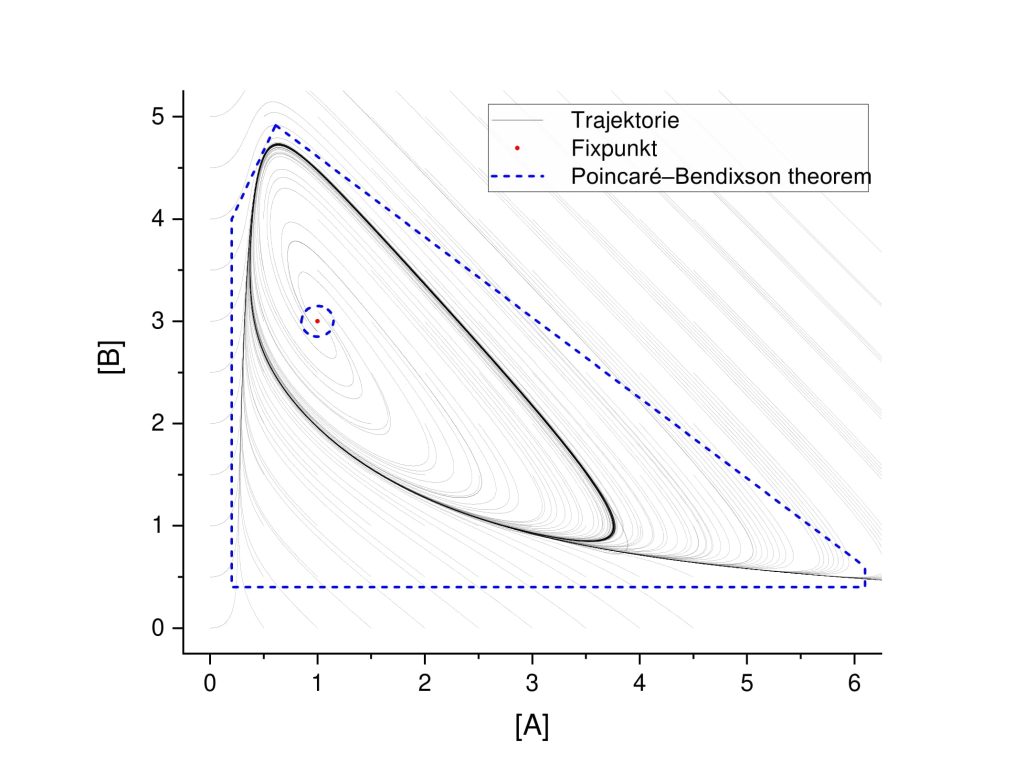
Reaction-Diffusion System of Brusselator
Both differential equations can now be advanced by using the second Fick’s law. ![\[\dfrac{\text{d} \left[X\right]}{\text{d} t} = k_1 \left[A\right] - k_2 \left[B\right] \left[X\right] + k_3 \left[X\right]^2 \left[Y\right] - k_4 \left[X\right] + D_x \nabla^2 \left[X\right] \]](https://lukaswittmann.com/wp-content/ql-cache/quicklatex.com-f27fdd4e1ff8dc90d87044277044d03a_l3.png "Rendered by QuickLaTeX.com")
![\[\dfrac{\text{d} \left[Y\right] }{\text{d} t} = k_2 \left[B\right] \left[X\right] - k_3 \left[X\right]^2 \left[Y\right] + D_y \nabla^2 \left[Y\right]\]](https://lukaswittmann.com/wp-content/ql-cache/quicklatex.com-3693f4a1b5502ebf49c45bed5fee1977_l3.png "Rendered by QuickLaTeX.com")
Dynamic Analysis of the Reaction-Diffusion System
It is found, that the Fixpoint equals the one of the spartially homogenous system. ![\[F=\left(\dfrac{k_1 \left[A\right]}{k_4} ,\; \dfrac{k_2 k_4 \left[B\right]}{k_3 k_1 \left[A\right]}\right)\]](https://lukaswittmann.com/wp-content/ql-cache/quicklatex.com-ad16b528aeef46ba3d2320f2c469f0b1_l3.png "Rendered by QuickLaTeX.com")
![\[\dfrac{\text{d} \left[X\right]}{\text{d} t} = k_1 \left[A\right] - k_2 \left[B\right] \left[X\right] + k_3 \left[X\right]^2 \left[Y\right] - k_4 \left[X\right] + D_x \nabla^2 \left[X\right] \quad\equiv\quad f\left([X],[Y]\right) + D_x \nabla^2 \left[X\right] \]](https://lukaswittmann.com/wp-content/ql-cache/quicklatex.com-2f322572ea6f8b3dbb9e67f213de7e8c_l3.png "Rendered by QuickLaTeX.com")
![\[\dfrac{\text{d} \left[Y\right] }{\text{d} t} = k_2 \left[B\right] \left[X\right] - k_3 \left[X\right]^2 \left[Y\right] + D_y \nabla^2 \left[Y\right] \quad\equiv\quad g\left([X],[Y]\right) + D_y \nabla^2 \left[Y\right]\]](https://lukaswittmann.com/wp-content/ql-cache/quicklatex.com-71e437cdf1159f23981875587b39d41a_l3.png "Rendered by QuickLaTeX.com")
 \: \Rightarrow \: [X]^*+\Delta [X](r,t)\: =\: [X]^* + \sin(\omega r + \phi)\Delta [X](t)\]](https://lukaswittmann.com/wp-content/ql-cache/quicklatex.com-abea89a0da1b2f45d6ab9bba3186b62c_l3.png "Rendered by QuickLaTeX.com")
 ,
, ![\dfrac{\delta [X]^*}{\delta t}=0](https://lukaswittmann.com/wp-content/ql-cache/quicklatex.com-4d43a11867dc8eb226740cf201da7ed5_l3.png "Rendered by QuickLaTeX.com") and
and 
![\[S\dfrac{\delta\Delta[X]}{\delta t}= f\left([X]^*+S\Delta[X],[Y]^*+S\Delta[Y]\right) - D_x \omega^2 S \Delta[X] \]](https://lukaswittmann.com/wp-content/ql-cache/quicklatex.com-69e378acad18e53685154732cf66abaa_l3.png "Rendered by QuickLaTeX.com")
![\[S\dfrac{\delta\Delta[Y]}{\delta t}= g\left([X]^*+S\Delta[X],[Y]^*+S\Delta[Y]\right) - D_y \omega^2 S \Delta[Y]\]](https://lukaswittmann.com/wp-content/ql-cache/quicklatex.com-dfd5f9c99b77c9afc55b3acf7da63d47_l3.png "Rendered by QuickLaTeX.com")
![\renewcommand{\arraystretch}{1.2}[C]=\begin{bmatrix} [X] \\ [Y] \end{bmatrix}](https://lukaswittmann.com/wp-content/ql-cache/quicklatex.com-c2bba7992cd84d9796b8b5d1b37ba1c3_l3.png "Rendered by QuickLaTeX.com") ,
, ![$\renewcommand{\arraystretch}{1.2}k\left([C]^*+\sin(\omega r + \phi)\Delta[C]\right)=\begin{bmatrix}f\left([X]^*+S\Delta[X],[Y]^*+S\Delta[Y]\right) \\ g\left([X]^*+S\Delta[X],[Y]^*+S\Delta[Y]\right) \end{bmatrix}](https://lukaswittmann.com/wp-content/ql-cache/quicklatex.com-cbdc1db88ee8d451d3ddd17bd1b137a4_l3.png "Rendered by QuickLaTeX.com") and
and 
![\[\sin(\omega r + \phi)\dfrac{\delta \Delta [C]}{\delta t}= k\left([C]^*+\sin(\omega r + \phi)\Delta[C]\right)-D\omega^2\sin(\omega r + \phi) \Delta[C]\]](https://lukaswittmann.com/wp-content/ql-cache/quicklatex.com-62ea12bbb2ccd0814531df2668ed8b88_l3.png "Rendered by QuickLaTeX.com")
![\[\renewcommand{\arraystretch}{2}k\left([C]^*+\sin(\omega r + \phi)\Delta[C]\right) \approx k\left([C]^*\right)+\begin{bmatrix}\dfrac{\delta f([X],[Y])}{\delta [X]} & \dfrac{\delta f([X],[Y])}{\delta [Y]}\\\dfrac{\delta g([X],[Y])}{\delta [X]} & \dfrac{\delta g([X],[Y])}{\delta [Y]} \end{bmatrix}\sin(\omega r + \phi)\Delta[C]\]](https://lukaswittmann.com/wp-content/ql-cache/quicklatex.com-35242ca5b9aa262d85dfacb864a6e5ae_l3.png "Rendered by QuickLaTeX.com")
![\[\sin(\omega r + \phi)\dfrac{\delta \Delta [C]}{\delta t}= \sin(\omega r + \phi) J_{g,f}\left(\left[X\right],\left[Y\right] \right)\Delta[C] - D\omega^2\sin(\omega r + \phi) \Delta[C]\]](https://lukaswittmann.com/wp-content/ql-cache/quicklatex.com-d1aa9e8b7e2215348e74dffad29b322f_l3.png "Rendered by QuickLaTeX.com")
![\[\dfrac{\delta \Delta [C]}{\delta t} = (J_{g,f}\left(\left[X\right],\left[Y\right] \right)-D\omega^2)\Delta[C]\]](https://lukaswittmann.com/wp-content/ql-cache/quicklatex.com-a45e4c59c3d5c3bd276a4ff884cfc8a9_l3.png "Rendered by QuickLaTeX.com")
![[C]^*](https://lukaswittmann.com/wp-content/ql-cache/quicklatex.com-026bbafb4d0300c9fbef3b98e303e69f_l3.png "Rendered by QuickLaTeX.com") can now be aproximated with the use of
can now be aproximated with the use of
![\[J_{g,f}\left(\left[X\right],\left[Y\right] \right)-D\omega^2 =\renewcommand{\arraystretch}{2}\begin{bmatrix}\dfrac{\delta f([X],[Y])}{\delta [X]} & \dfrac{\delta f([X],[Y])}{\delta [Y]}\\\dfrac{\delta g([X],[Y])}{\delta [X]} & \dfrac{\delta g([X],[Y])}{\delta [Y]}\end{bmatrix} - \begin{bmatrix} D_x\omega^2 & 0 \\ 0 & D_y\omega^2 \end{bmatrix} \text{.}\]](https://lukaswittmann.com/wp-content/ql-cache/quicklatex.com-b2f28221377340e0553a1e5e7db21708_l3.png "Rendered by QuickLaTeX.com")
 –
– -phase space.
![\[D_{y}^{grenz,1}\left([A],[B],D_x \right) = \dfrac{\left([B]+1\pm 2\sqrt{[B]}\right)[A]^2D_x}{[B]^2-2[B]+1}\]](https://lukaswittmann.com/wp-content/ql-cache/quicklatex.com-d8179b6ddff4689127101926607b6f0a_l3.png "Rendered by QuickLaTeX.com")
![\[D_{y}^{grenz,2}\left(D_x \right) = D_x\]](https://lukaswittmann.com/wp-content/ql-cache/quicklatex.com-f7b341eba187446754f28dc5eeb25afe_l3.png "Rendered by QuickLaTeX.com")
![\[[B]_H\left([A]\right) = [A]^2+1 \]](https://lukaswittmann.com/wp-content/ql-cache/quicklatex.com-bc14426892726e7b457d1ccf9a068727_l3.png "Rendered by QuickLaTeX.com")
![\[[B]_T\left([A],D_x,D_y \right) = \left(1+[A]\sqrt{\dfrac{D_x}{D_y}}\right)^2]\]](https://lukaswittmann.com/wp-content/ql-cache/quicklatex.com-923f74acff77d20629d8f295991b42b4_l3.png "Rendered by QuickLaTeX.com")

![[A] = 1](https://lukaswittmann.com/wp-content/ql-cache/quicklatex.com-4e892a87cb1b7281d84049fc1e1f05a6_l3.png "Rendered by QuickLaTeX.com") und
und ![[B]=3](https://lukaswittmann.com/wp-content/ql-cache/quicklatex.com-93282da6e67f258cdef855bbb5da3031_l3.png "Rendered by QuickLaTeX.com") , welche stabile Fixpunkte und instabile Fixpunkte liefern sowie die Turing-Stabilität
, welche stabile Fixpunkte und instabile Fixpunkte liefern sowie die Turing-Stabilität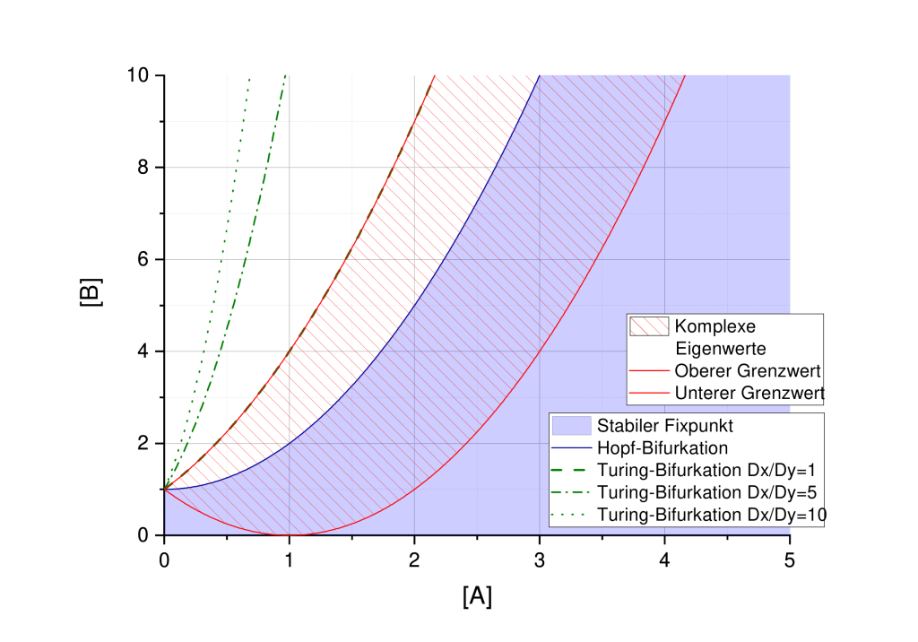
 ,
,  , and
, and  , which provide stable fixed points and unstable fixed points, and Turing stability.
Leave a Reply